library(terra)
# we import the bands
b2 <- rast('./Data_RS/Lahore_2025-09-16_LC91490382025259LGN00_B2.tif')
b3 <- rast('./Data_RS/Lahore_2025-09-16_LC91490382025259LGN00_B3.tif')
b4 <- rast('./Data_RS/Lahore_2025-09-16_LC91490382025259LGN00_B4.tif')
b5 <- rast('./Data_RS/Lahore_2025-09-16_LC91490382025259LGN00_B5.tif')
b6 <- rast('./Data_RS/Lahore_2025-09-16_LC91490382025259LGN00_B6.tif')
b7 <- rast('./Data_RS/Lahore_2025-09-16_LC91490382025259LGN00_B7.tif')Remote sensing analysis
Objectives of the fifth section
The aim of this section is to learn how to perform some remote sensing operations using R. We will take the example of the Lahore region and characterise its territory in 2025 using a Landsat image. In this section, we will cover the following points:
- importing a spectral band into R via terra
- exporting a raster from R to a geoTiff
- renaming a raster
- raster calculation to recalibrate a Landsat image
- calculation of radiometric indices for vegetation and water
- supervised classification of land cover
- validation of a classification raster
- calculating spectral signatures
We will classify land use into 7 classes (Table 1).
| id_class | label_class Colour | |
|---|---|---|
| 1 | Clear water | #0058ff |
| 2 | Turbid water | #2be2f9 |
| 3 | Dense vegetation | #188e00 |
| 4 | Wet vegetation | #0ccd19 |
| 5 | Dense built-up area | #a01300 |
| 6 | Diffuse built-up area | #f18873 |
| 7 | Bare soil | #b2b2b2 |
Data provided
For this exercise, we will use the data provided in the Data_RS directory: - Lahore_2025-09-16_LC91490382025259LGN00_B2.tif/B7.tif: spectral bands 2 to 7 of the Landsat 9 image from 16 September 2025 - train_2025.gpkg: training polygons for land cover classification - valid_2025.gpkg: validation polygons for land cover classification
These data are stored in the folder Data_RS available at this link.
Landsat images provided
For this example, we are using only 7 Landsat spectral bands out of the 11 normally available. In addition, the images used have been cropped and centred on Lahore in order to reduce their size.
Importing, calibrating and exploring images
We will begin by loading the six spectral bands provided into R. We import them using the terra library in the form of spatRaster objects.
The rasters now have more explicit names. We continue by importing the polygon vector files that we will use for training (train_2025.gpkg) and validation (valid_2025.gpkg). The RStoolbox library that we will use for classification needs to take vector objects in sf format as input. We therefore load these two layers in sf format.
Vector layers for the classification
These two layers were digitised manually in GIS software (e.g. QGIS) by visually interpreting land use. Several representative polygons must be taken for each class. These polygons must be large enough to take into account the heterogeneity of the classes but small enough to take only one class at a time. Care must also be taken not to overlap the training polygons and the validation polygons.
library(sf)
# import of the train and valid layers
train_poly <- st_read('./Data_RS/train_2025.gpkg')
Reading layer `train_2025' from data source
`/home/poulpe/Enseignement/hors_UP/LCWU_online/R_for_Geomatics/Data_RS/train_2025.gpkg'
using driver `GPKG'
Simple feature collection with 29 features and 1 field
Geometry type: POLYGON
Dimension: XY
Bounding box: xmin: 386034 ymin: 3454060 xmax: 460083 ymax: 3520876
Projected CRS: WGS 84 / UTM zone 43Nvalid_poly <- st_read('./Data_RS/valid_2025.gpkg')Reading layer `valid_2025' from data source
`/home/poulpe/Enseignement/hors_UP/LCWU_online/R_for_Geomatics/Data_RS/valid_2025.gpkg'
using driver `GPKG'
Simple feature collection with 26 features and 1 field
Geometry type: POLYGON
Dimension: XY
Bounding box: xmin: 396364.4 ymin: 3456851 xmax: 473111.4 ymax: 3518307
Projected CRS: WGS 84 / UTM zone 43NThe Landsat images provided are L2A level images, which means they are surface reflectances, essential for mapping land cover and calculating radiometric indices. However, as explained in the Landsat documentation, before using them, each spectral band must be recalibrated by applying multiplicative and additive parameters. The formula to be applied to each spectral band is as follows.
\[ SR = (DN \times 0.0000275) - 0.2 \]
Where DN corresponds to uncalibrated spectral bands.
# recalibration of the bands
b2 <- 0.0000275 * b2 - 0.2
b3 <- 0.0000275 * b3 - 0.2
b4 <- 0.0000275 * b4 - 0.2
b5 <- 0.0000275 * b5 - 0.2
b6 <- 0.0000275 * b6 - 0.2
b7 <- 0.0000275 * b7 - 0.2
At this stage, the loaded rasters have retained the names of the original geoTiff files, which will not be practical for the next steps. We will rename them with more relevant names.
# we renamne the rasters
names(b2) <-'sr_blue'
names(b3) <-'sr_green'
names(b4) <-'sr_red'
names(b5) <-'sr_nir'
names(b6) <-'sr_mir1'
names(b7) <-'sr_mir2'
We can then create a multi-band raster (a stack) that will allow us to build colour compositions in order to explore our images and our study area qualitatively. For example, we will create a false colour composition in which we associate the colour red with the near-infrared band, the colour green with the green band, and the colour blue with the blue band. In this type of composition, surfaces that reflect a lot in the near infrared and less in the green and blue bands will appear red. This is mainly vegetation that reflects in this way. Ultimately, in this type of colour composition, the pixels that appear red are mainly vegetation pixels.
# the multi-band raster
lt_stack <- c(b2, b3, b4, b5, b6, b7)

# we plot a false color composite
plotRGB(lt_stack, r=4, g=2, b=1, stretch='hist')
Explain the parameters passed to the plotRGB function
Answer
r, g and b designate the colours to be used to colour the spectral bands (red, green and blue). The numbers 4, 2 and 1 are the bands in the order in which they appear in the multi-band raster constructed previously. The stretch allows the contrasts of the colour composition to be optimised.
Spectral indices
Spectral indices are commonly used in remote sensing to highlight certain types of land cover, such as vegetation, water, bare soil, turbidity, snow, etc. Spectral indices are simple raster calculations that allow you to create a new raster highlighting the desired land cover, based on spectral bands. Here, we will use two indices, the first to characterise vegetation and the second to detect water surfaces.
NDVI
For vegetation, we will calculate the NDVI. This is undoubtedly the most widely used index. It is calculated by combining the near infrared and red bands and is calculated using the following formula.
\[ $NDVI = \frac{(NIR - Red)}{(NIR + Red)}$ \]
The result varies between -1 and +1. The closer a pixel is to 1, the more that pixel is covered by vegetation. The closer a pixel is to 0, while remaining positive, the more that pixel is covered by bare ground (natural or artificial). Finally, a negative pixel is often a pixel covered by water. The calculation is done simply in R.
# we calculate the NDVI
ndvi <- (b5 - b4)/(b5 + b4)
# we rename the raster of ndvi
names(ndvi) <- ndvi
plot(ndvi)
We can extract all pixels covered by vegetation by extracting pixels with an NDVI greater than 0.35. This gives us a binary raster where pixels covered by vegetation are set to 1 and the others to 0.
# we threshold the ndvi
veg <- ndvi > 0.35
names(veg) <- 'vegetation'
plot(veg)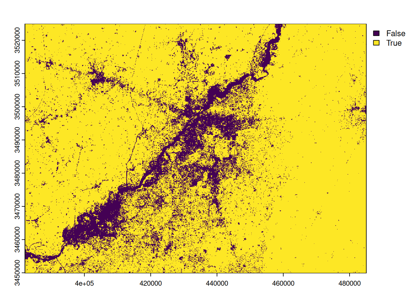
We can then convert this binary raster into a polygon and select the polygon corresponding to the vegetation.
# conversion into polygons
veg_vect <- as.polygons(veg, aggregate=TRUE)
# selection of the polygons of vegetation
veg_vect <- veg_vect[veg_vect$vegetation == 1,]
We may export the raster of NDVI and the polygons of vegetation.
# export of the layers
writeRaster(ndvi, './Data_processed/ndvi_2025.tif', overwrite=TRUE)
writeVector(veg_vect, './Data_processed/vegetation_2025.gpkg', overwrite=TRUE)
MNDWI
To extract water surfaces, we will use the MNDWI index. It is calculated by combining the green and mid-infrared bands using the following formula.
\[ MNDWI = \frac{(Green - SWIR1)}{(Green + SWIR1)} \]
The resulting raster varies between -1 and +1. All negative pixels are assumed to be water pixels. If the water is turbid, this threshold may be slightly positive. The calculation is done simply in R.
# we calculate the MNDWI
mndwi <- (b6 - b3)/(b6 + b3)
# we rename the raster of MNDWI
names(mndwi) <- mndwi
plot(mndwi)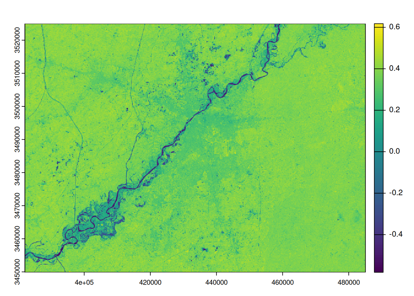
We can extract all pixels covered by water by extracting pixels with an MNDWI below than 0. This gives us a binary raster where pixels covered by water are set to 1 and the others to 0.
# we threshold the mndwi
water <- mndwi < 0
names(water) <- 'water'
plot(water)
We can then convert this binary raster into a polygon and select the polygon corresponding to the water.
# conversion into polygons
water_vect <- as.polygons(water, aggregate=TRUE)
# selection of the polygons of water
water_vect <- water_vect[water_vect$water == 1,]
We may export the raster of MNDWI and the polygons of water.
# export of the layers
writeRaster(mndwi, './Data_processed/mndwi_2025.tif', overwrite=TRUE)
writeVector(water_vect, './Data_processed/water_2025.gpkg', overwrite=TRUE)
Supervised Classification
We can now perform supervised classification of land cover in our study area. We will perform classification according to the seven classes presented at the beginning of this section. We will classify our multiband raster containing the six Landsat spectral bands provided using the training polygons provided in the train_poly layer. We will use the random forest classification algorithm. We will validate this classification using the valid_poly layer.
Classification is performed using the superclass function from the RStoolbox library. At the end of this classification process, we obtain an object containing the classification results, such as the confusion matrix, performance indicators, and the classification raster.
library(RStoolbox)
# supervised classification using the function superclass of the library RStoolbox
sc <- superClass(lt_stack, train_poly, valid_poly, responseCol = "id_class", model = "rf")
#sc
The classification confusion matrix can be easily retrieved.
# confusion matrix
sc$validation$performance$table
Reference
Prediction 1 2 3 4 5 6 7
1 227 0 0 0 0 0 0
2 0 872 0 0 0 0 0
3 0 0 332 45 0 0 0
4 0 0 0 125 0 0 0
5 0 0 0 0 828 0 0
6 0 0 0 0 24 846 60
7 0 0 0 0 3 5 375It is possible to retrieve quality indicators by class.
# accuracy assessment by class
sc$validation$performance$byClass
Sensitivity Specificity Pos Pred Value Neg Pred Value Precision
Class: 1 1.0000000 1.0000000 1.0000000 1.0000000 1.0000000
Class: 2 1.0000000 1.0000000 1.0000000 1.0000000 1.0000000
Class: 3 1.0000000 0.9868035 0.8806366 1.0000000 0.8806366
Class: 4 0.7352941 1.0000000 1.0000000 0.9875588 1.0000000
Class: 5 0.9684211 1.0000000 1.0000000 0.9907344 1.0000000
Class: 6 0.9941246 0.9709443 0.9096774 0.9982219 0.9096774
Class: 7 0.8620690 0.9975809 0.9791123 0.9821375 0.9791123
Recall F1 Prevalence Detection Rate Detection Prevalence
Class: 1 1.0000000 1.0000000 0.06066275 0.06066275 0.06066275
Class: 2 1.0000000 1.0000000 0.23303046 0.23303046 0.23303046
Class: 3 1.0000000 0.9365303 0.08872261 0.08872261 0.10074826
Class: 4 0.7352941 0.8474576 0.04543025 0.03340460 0.03340460
Class: 5 0.9684211 0.9839572 0.22848744 0.22127205 0.22127205
Class: 6 0.9941246 0.9500281 0.22741849 0.22608231 0.24853020
Class: 7 0.8620690 0.9168704 0.11624800 0.10021379 0.10235168
Balanced Accuracy
Class: 1 1.0000000
Class: 2 1.0000000
Class: 3 0.9934018
Class: 4 0.8676471
Class: 5 0.9842105
Class: 6 0.9825344
Class: 7 0.9298249Finally, we can retrieve the raster resulting from the classification in a terra object.
# the classification raster
classif <- sc$map
names(classif) <- 'classif_2025'
classif
class : SpatRaster
dimensions : 2504, 3433, 1 (nrow, ncol, nlyr)
resolution : 30, 30 (x, y)
extent : 382065, 485055, 3449865, 3524985 (xmin, xmax, ymin, ymax)
coord. ref. : WGS 84 / UTM zone 43N (EPSG:32643)
source(s) : memory
name : classif_2025
min value : 1
max value : 7 We may map it.
# map of the classification raster
# the label of the classes
label_classes <- c("Clear water", "Turbid water", "Dense vegetation", "Wet vegetation", "Dense built-up",
                  "Diffuse built-up", "Bare soil")
# the colors of the classes
# définition des couleurs pour chaque classe dans (dans l'ordre des id de classe)
pal_col <- c("#0058ff",
             "#2be2f9",
             "#188e00",
             "#0ccd19",
             "#a01300",
             "#f18873",
             "#b2b2b2")
# association of the labels to the id of the classes
levels(classif) <- data.frame(c(1, 2, 3, 4, 5, 6, 7),
                                 classe = label_classes)

# création de la carte
plot(classif,
     col = pal_col,
     type = "classes",
     main = "Land cover of the Lahore area (2025)",
     axes = FALSE,
     legend = TRUE,
     plg = list(title = "Land cover",
                cex = 1,
                x = "bottomright",
                bty = 'o',
                bg = "#ececec",
                box.col = "#ececec"))
north()
sbar(d = 20000,
     label = c("20 km")
)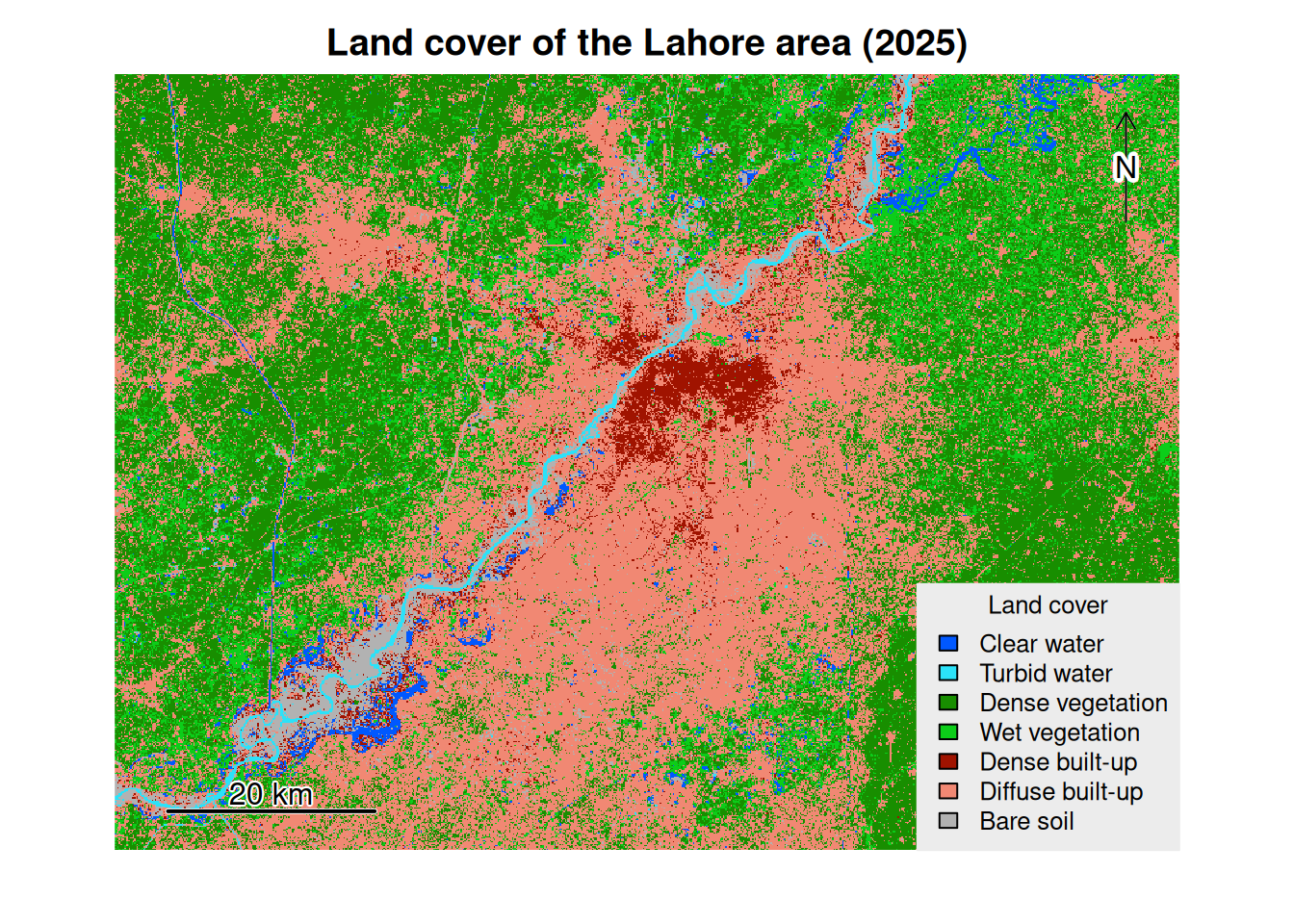
We can calculate a zonal histogram, also known as a unique value report, to find out how many pixels belong to each class. Knowing the spatial resolution of a pixel, it is possible to calculate the area occupied by each land cover class.
# we calculate the zonal histogram of the classification
report <- freq(classif)
# we store it as a dataframe
report <- as.data.frame(report)
# we grab the X and Y resolution of the raster
x_res <- res(classif)[[1]]
y_res <- res(classif)[[2]]
# we calculate the area of one pixel
pix_area <- x_res * y_res
# we add a column of area in the dataframe by multiplying the count by the size of one pixle
report$area_km2 <- report$count * pix_area / 1000000
report
layer value count area_km2
1 1 Clear water 157007 141.3063
2 1 Turbid water 64905 58.4145
3 1 Dense vegetation 3219978 2897.9802
4 1 Wet vegetation 1250498 1125.4482
5 1 Dense built-up 250704 225.6336
6 1 Diffuse built-up 3364819 3028.3371
7 1 Bare soil 288321 259.4889The dominant land use class is Diffuse built-up class , covering an area of 3028.34 km2. Thanks to this report, we can draw a bar chart to visualize the respective share of each land cover class.
library(plotly)
# the barplot
fig <- plot_ly(report, x = ~value, y = ~area_km2, type = 'bar',
        # we set the colors of the bars as the ones used in the classification
        marker = list(color = c('#0058ff', '#2be2f9',
                                '#188e00', '#0ccd19',
                                '#a01300', '#f18873',
                                '#b2b2b2')))
        # we arrange the order of the bars
fig <- fig  %>% layout(xaxis = list(categoryorder = "array",
                    categoryarray = c("Clear water", "Turbid water", "Dense vegetation", "Wet vegetation", "Dense built-up",
                                      "Diffuse built-up", "Bare soil")))
        # we define the titles
fig <- fig %>% layout(title = "Land cover in the area of Lahore (2025)",
         xaxis = list(title = "Land cover classes"),
         yaxis = list(title =  "Area (km<sup>2</sup>)"))
fig