library(terra)
# divisions with population and density
pk_div_pop <- vect('./Data_bonus/divisions_PK_pop.gpkg')
# main waterways
hydro <- vect('./Data/main_rivers_PK.gpkg')
# the DEM
dem <- rast('./Data/GTopo_PK.tif')
# land cover of the Hazara division
land_cover_hazara<- rast('./Data_bonus/land_cover_hazara.tif')Thematic mapping
Objectives of the third section
This third section presents some thematic map layout features with R, both vector and raster. We will mainly use the mapsf library. Start by installing this library if you have not already done so. By the end of this third section, you will be able to create the following maps:
- map with labels
- choropleth map for a quantitative variable
- proportional circle map for a quantitative stock variable
- map for a discrete raster
- map for a continuous raster
Data to be represented
We will now represent the demographic data (population, density) that we explored earlier. With regard to the raster, we will focus on land use and topography. We will begin by loading the layers we will need, if they are not already loaded.
Location map
To begin with, we will simply map the divisions with their labels. The mapsf library, for vectors, only supports the sf format. It is therefore necessary to convert our terra vector objects into sf objects. Fortunately, this is very easy to do.
library(mapsf)
library(sf)
# we convert the divisions into a sf object
pk_div_pop_sf <- st_as_sf(pk_div_pop)

# we define the credits
credits <- paste0("Sources: Bureau of Statistics, 2025\n", "mapsf ", packageVersion("mapsf"))

# map of the divisions
mf_map(pk_div_pop_sf, col = "#e4e9de", border = "darkseagreen4") # we define the style
# plotting of the labels
mf_label(
  x = pk_div_pop_sf,                             # the layer to map
  var = "NAME_2",                                # the field containing the labels
  cex = 0.5,
  font = 4,                                      # the size of the labels
  halo = TRUE,                                   # put a halo around labels
  r = 0.1,
  overlap = FALSE,                               # do not allow overlapping labels
  q = 3,
  lines = FALSE
)
# framwork
mf_title("The Divisions of Pakistan")            # the title of the map
mf_credits(credits)                              # plotting of the credits
mf_arrow(pos = "topright")                       # North arrow at the top right
mf_scale()                                       # the scale bar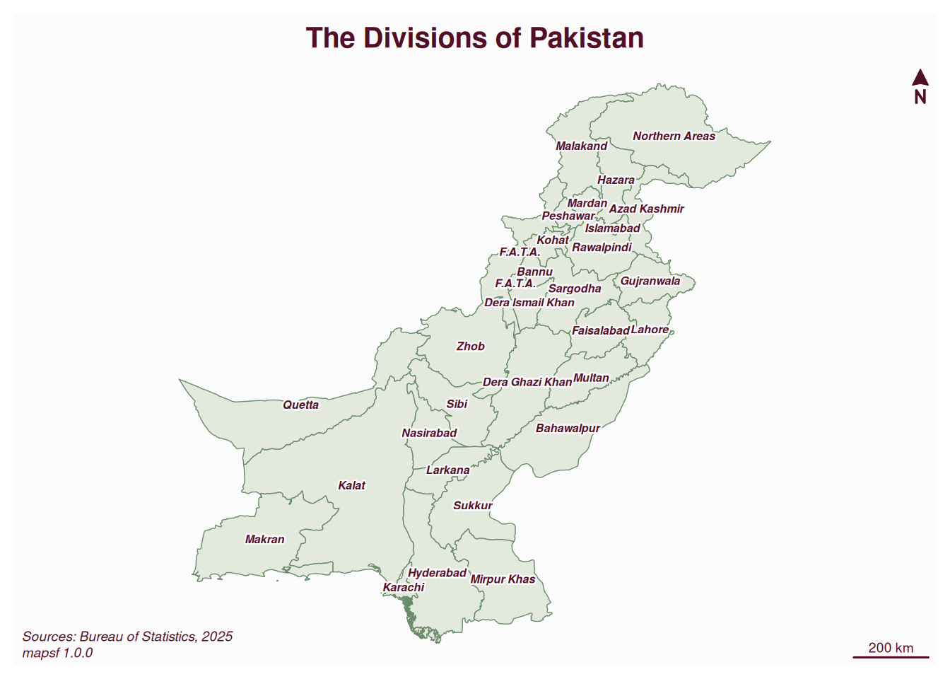
When the map is small, it can look cluttered.
We can include a location inset (called an inset) in our map for a pro touch. We can put any layer we want in it, but here we will use a predefined inset from the package showing a globe and the location on it.
# map of the divisions
mf_map(pk_div_pop_sf, col = "#e4e9de", border = "darkseagreen4") # we define the style
# plotting of the labels
mf_label(
  x = pk_div_pop_sf,                             # the layer to map
  var = "NAME_2",                                # the field containing the labels
  cex = 0.5,
  font = 4,                                      # the size of the labels
  halo = TRUE,                                   # put a halo around labels
  r = 0.1,
  overlap = FALSE,                               # do not allow overlapping labels
  q = 3,
  lines = FALSE
)
# framwork
mf_title("The Divisions of Pakistan")            # the title of the map
mf_arrow(pos = "topright")                       # North arrow at the top right
mf_scale()
mf_inset_on(x = "worldmap", pos = "bottomleft") # définition de l'inset
mf_worldmap(x = pk_div_pop_sf)                     # on centre l'inset sur notre couche
mf_inset_off()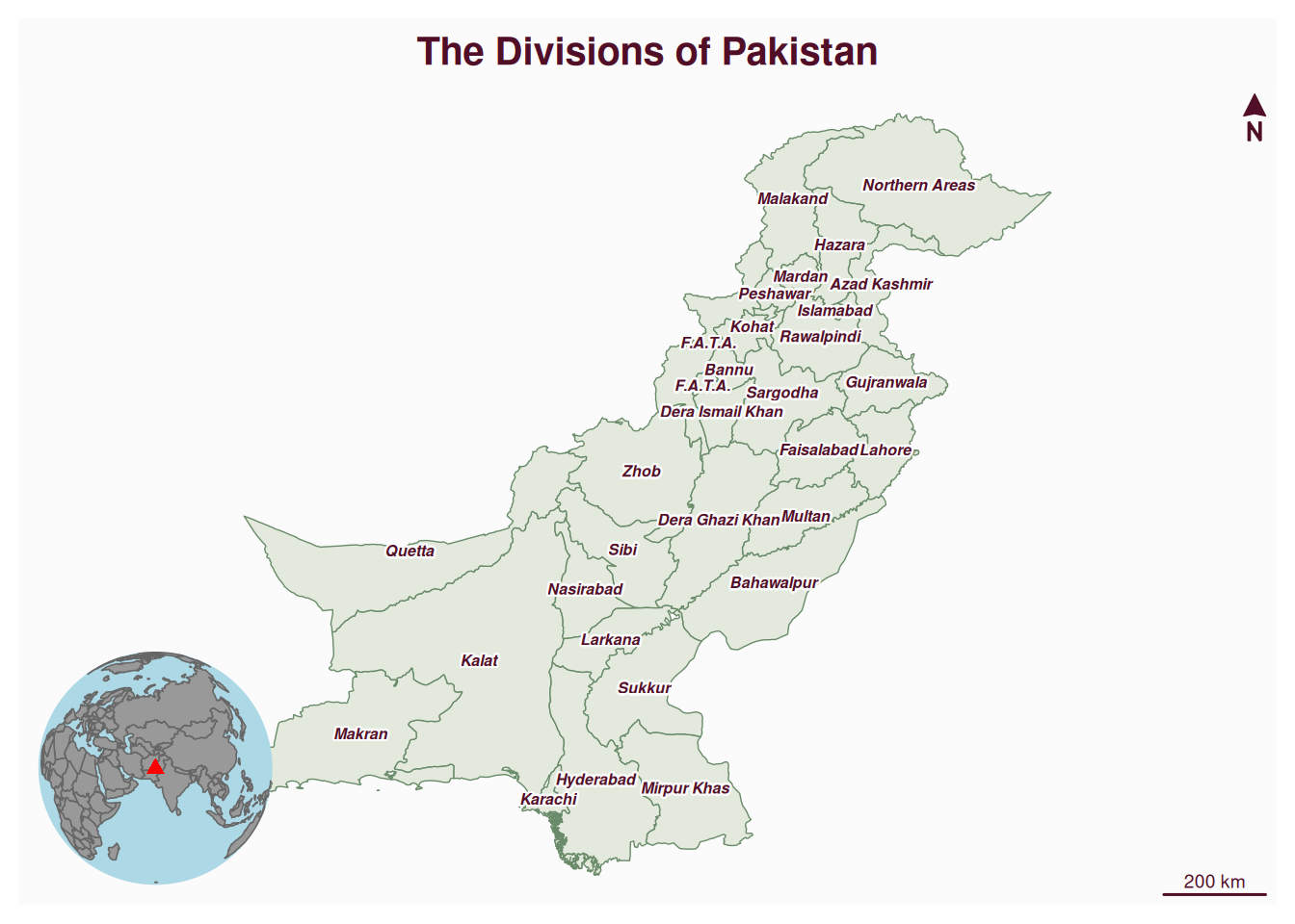
Choropleth map
We will now map population densities of the divisions. This is a quantitative ratio variable. We will therefore use flat colours and varying shades.
# mapping of the population densities per division
mf_map(
  x = pk_div_pop_sf,                            # the layer to map
  var = "density_inh",                          # the field to map
  type = "choro",                               # we ask for a choropleth map
  breaks = "geom",                              # method of discretisation
  nbreaks = 5,                                  # number of classes
  pal = "Teal",                                 # the palette to use
  border = "white",                             # the color of the boundaries of the divisions
  lwd = 0.5,                                    # width of the boundaries
  leg_pos = "bottomleft",                       # position of the legend
  leg_adj = c(0, 3),
  leg_title = "Pop density \n(inh. / km2)"      # title of the legend
)
mf_title("High densities along the Indus River")
mf_credits(credits)
mf_arrow()
mf_scale()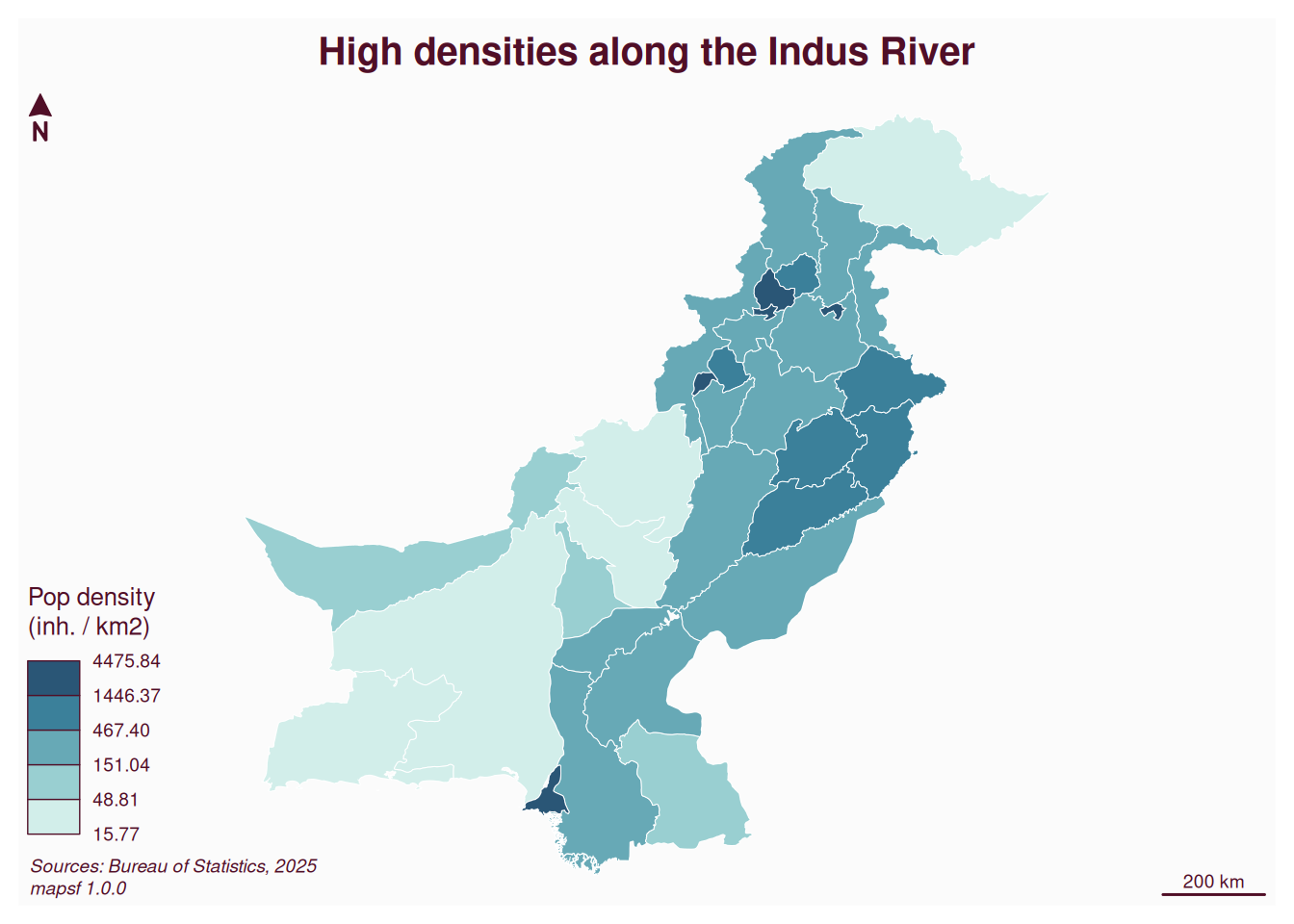
Proportional circle map
We will now represent the number of inhabitants per division. We are now dealing with a quantitative stock variable. We will therefore use the proportional circle.
# map of the population per division
mf_map(pk_div_pop_sf)
mf_map(
  x = pk_div_pop_sf,                       # the layer to map
  var = "Census_2017",                     # the field to map
  type = "prop",                           # we ask for proportional circles
  inches = 0.2,                            # we define the size of smallest circle
  col = "brown4",                          # the color of the circles
  leg_pos = "topright",                    # the position of the legend
  leg_adj = c(0, -3),
  leg_title = "Nb inh."                    # the title of the legend
)
# habillage
mf_title("Unevenly populated divisions")
mf_credits(credits)
mf_arrow()
mf_scale()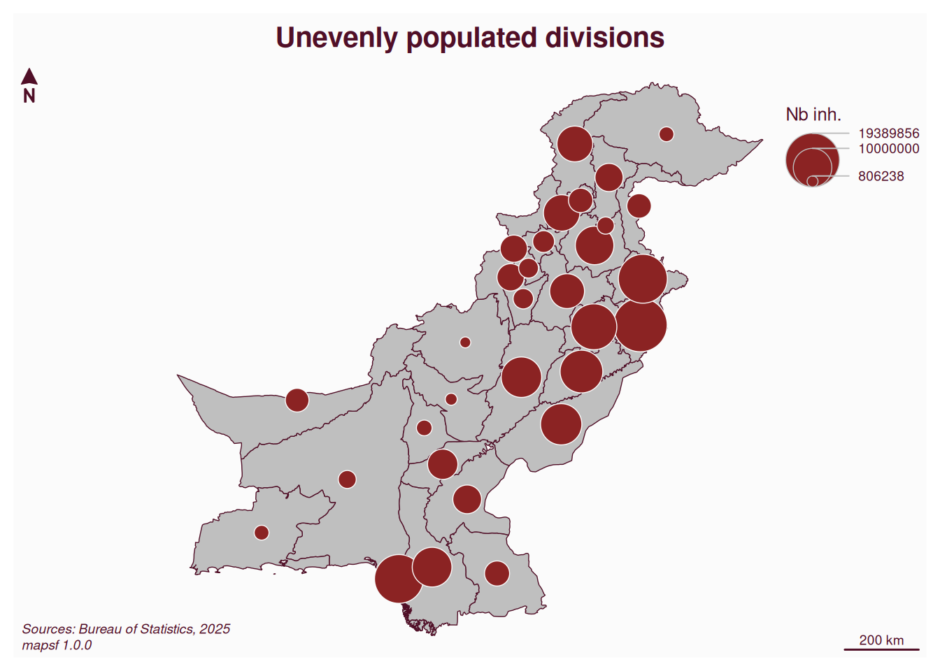
Your turn
Produce these three maps for a district of your choice.
Continuous raster map
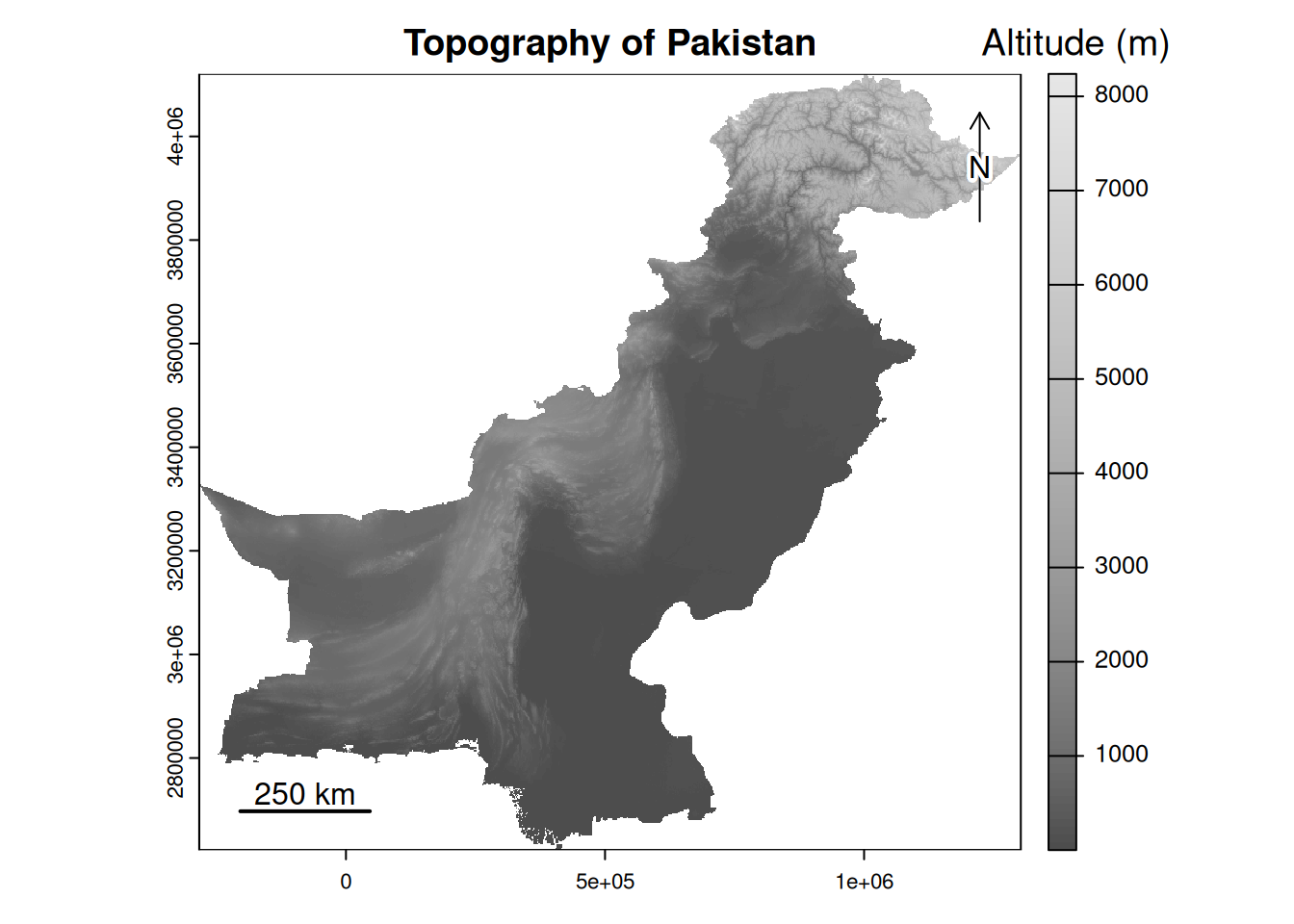
By continuous raster, we mean rasters whose values are continuous, such as altitude, temperature, NDVI values, etc. To map this type of raster, we can stay within the terra library. Here, we will represent the topography of Pakistan.
# map of the topography
plot(dem,                                     # the raster to map
     col=gray.colors(100),                    # the color palette
     main='Topography of Pakistan',           # the title of the map
     plg=list(                                # params for the legend
        title = "Altitude (m)",               # the title of the legend
        title.cex = 1.2,                      # the size of the title legend
        cex = 1)                              # the size of the text of the title legend
    )
# we add a North arrow
terra::north()
# we add a scale bar (with a distance of 250 km) and a relevant label
terra::sbar(d = 250000,
     label = c("250 km")
)
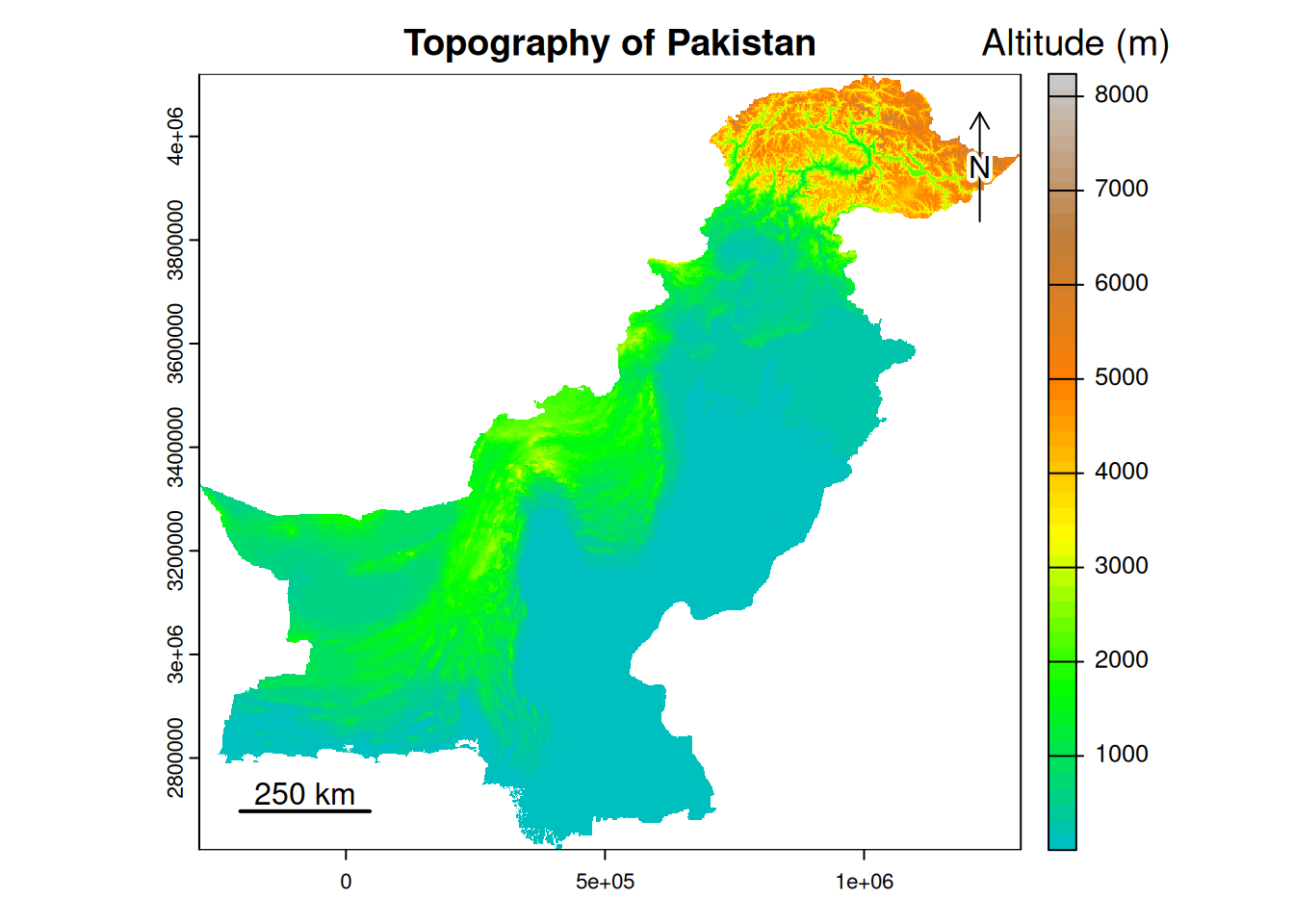
We can change the colour palette and use the one dedicated to altitude, called elevation.
# map of the topography
plot(dem,                                     # the raster to map
     col=map.pal("elevation"),                # the color palette
     main='Topography of Pakistan',           # the title of the map
     plg=list(                                # params for the legend
        title = "Altitude (m)",               # the title of the legend
        title.cex = 1.2,                      # the size of the title legend
        cex = 1)                              # the size of the text of the title legend
    )
# we add a North arrow
terra::north()
# we add a scale bar (with a distance of 250 km) and a relevant label
terra::sbar(d = 250000,
     label = c("250 km")
)
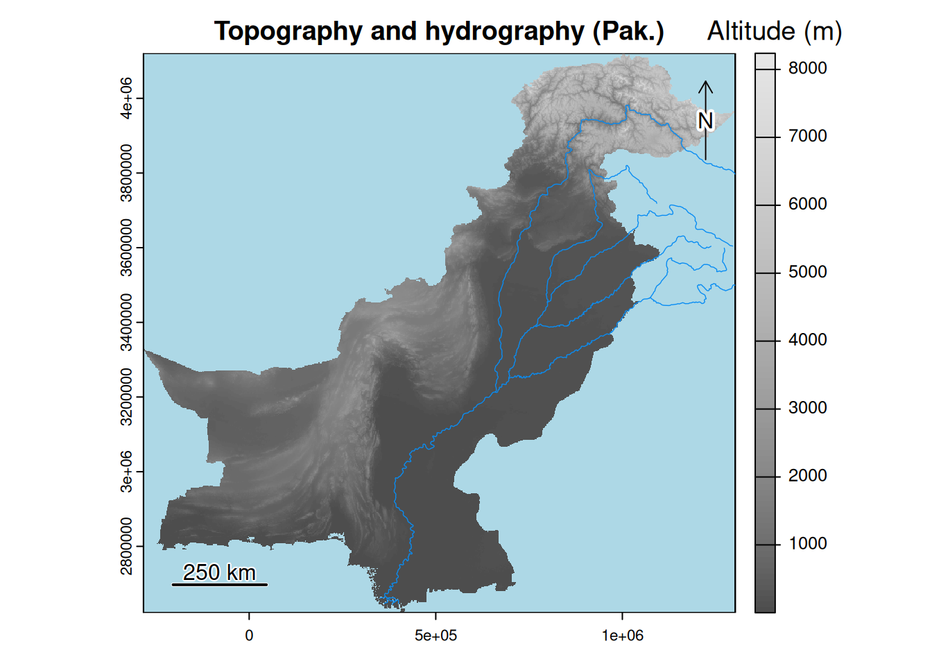
It is possible to add vector data to our map. For example, we will add the main rivers to our map.
# we import the layer of the main waterways
hydro <- vect('./Data/main_rivers_PK.gpkg')
# we reproject the layer in WGS84/UTM Zone 42 North
hydro <- project(hydro, 'EPSG:32642')

# map of the topography and the main waterways
plot(dem,
     col=gray.colors(100),
     main='Topography and hydrography (Pak.)',
     plg=list(
        title = "Altitude (m)",
        title.cex = 1.2,
        cex = 1),
     background = "lightblue"  # we add a blue background
    )
lines(hydro,                   # we add the waterways
      col='#088cf3',           # we define the color of the rivers in hexadecimal
      lwd=0.7)                 # we define the width of the lines
north()
sbar(d = 250000,
     label = c("250 km")
)
Discrete raster map
By discrete raster, we mean a raster whose values can only take on a certain range. This is the case for land cover rasters, for example. Here, we will map land cover for the Hazara division.
# we grab the boundaries of the selected divisions
div_hazara <- pk_div_pop[pk_div_pop$NAME_2 == 'Hazara', ]

# we define the labels of the land covers classes (in the order of the id classes)
# only the classes actually present on our raster are selected
labels_classes <- c("Espace boisé", "Broussailles", "Prairie", "Culture", "Bâti",
                  "Sol nu/Vég. éparse", "Neige et glace", "Eau", "Zone humide", "Mousses")

# we define the colors of each class (in the order of the id classes)
pal_col <- c("#006400",
             "#ffbb22",
             "#ffff4c",
             "#f096ff",
             "#fa0000",
             "#b4b4b4",
             "#f0f0f0",
             "#0064c8",
             "#0096a0",
             "#fae6a0")

# we associate the names of the classes to their id
levels(land_cover_hazara) <- data.frame(c(10, 20, 30, 40, 50, 60, 70, 80, 90, 100),
                                 classes = labels_classes)
par(mar = c(3, 3, 3, 8), xpd = TRUE)
# we create the map
plot(land_cover_hazara,                       # the raster to map
     col = pal_col,                           # the color palette to be used
     type = "classes",                        # we ask for a map in categories
     main = "Land cover in Hazara",           # the title of the map
     axes = FALSE,                            # we do not draw the axis of the projection
     legend = TRUE,
     # we define the legend
     plg = list(title = "Land cover",         # the title of the legend
                cex = 1,                      # the size of the text
                x = "bottomright",            # the position of the legend
                bg = "#eaeae",                # the color of the background of the legend (do not work??)
                box.col = "black"))           # the color of the frame of the legend (do not work??)
lines(div_hazara,                             # we add the boundaries of the division
      col='#eaeaea',                          # the colour of the boundaries in hexadecimal
      lwd=3)                                  # the with of the boundaries
north()
sbar(d = 20000,
     label = c("20 km")
     )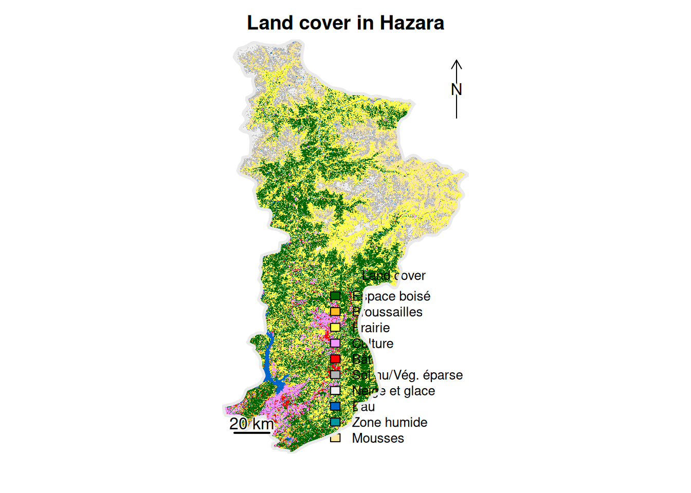
The rendering could be improved, the option for the caption background colour does not seem to work… but the essentials are there.