Geoprocessings and Rasters

Objectives of the second section

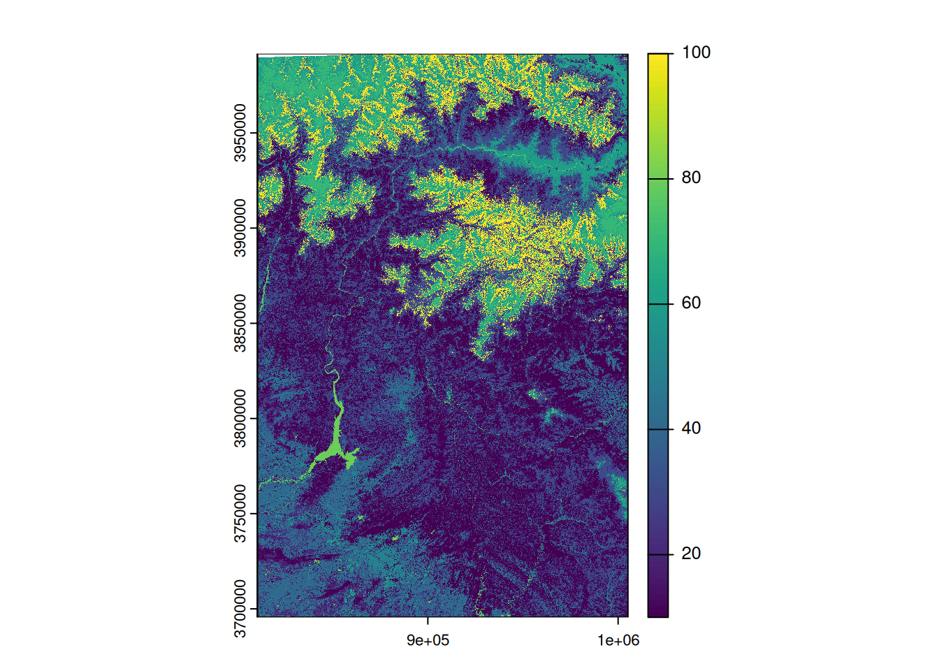
The aim of this second part is to manipulate several vector layers using geoprocessing in order to extract additional information. We will also take this opportunity to perform some basic manipulations on raster files. By the end of this part, you will be able to perform the following manipulations with R:

import a raster into R via terra
export a raster
calculate zonal statistics on a raster
reproject a raster
cutting and masking a raster according to a mask layer
vectorising a raster
automating tasks

The fisrt theme of this section will be to determine, for a given district, the division with the largest proportion of wooded area in relation to its total surface area. The second theme of this section will be to characterise (briefly) the topography at the scale of Pakistani districts. In particular, we will see how to calculate maximum and average altitudes automatically.

Data provided

For this exercise, we will use the following data provided:

the layer of the districts of Pakistan (PK_admin_L2.gpkg see first part)
the 2021 land cover raster layer for a portion of Pakistan (ESA_WorldCover.tif)
a national-scale DTM (GTopo_PK.tif)

The land cover layer ESA WorldCover is a raster showing land cover for the entire world at a spatial resolution of 10 m. For the purposes of this example, only a small extract for a part of Pakistab is provided, and this extract has been resampled to a resolution of 50 m in order to reduce the file size. The nomenclature is as follows (@#tbl-esa):

Table 1: ESA World Cover nomenclature.
Class ID	Class	Colour
10	Wooded area	#006400
20	Scrubland	#ffbb22
30	Grassland	#ffff4c
40	Cropland	#f096ff
50	Built-up area	#fa0000
60	Bare ground / Sparse vegetation	#b4b4b4
70	Snow and ice	#f0f0f0
80	Permanent water	#0064c8
90	Grassland wetland	#0096a0
95	Mangrove	#00cf75
100	Moss and lichen	#fae6a0

Importing, exploring and reprojecting a raster

We will start by importing our land cover raster into R via terra. This will give us a spatRaster object.

library(terra)
# import of the land cover
land_cover <- rast('./Data/ESA_WorldCover.tif')
# plotting
plot(land_cover)

We can explore some useful properties of this layer, such as the spatial resolution and the coordinate reference system (CRS) used.

# extraction of the spatial resolution of the raster (X and Y)
res_X <- res(land_cover)[1]
res_Y <- res(land_cover)[2]

What is the shape of the pixels on our raster? What are the dimensions of this shape?

# extraction of the CRS with all the details
scr_rast <- crs(land_cover, describe=T)
# extraction of the EPSG code only
epsg_rast <- crs(land_cover, describe=T)$code

Can you directly compare this layer with your division layer?

Answer

Yes, the CRS are the sames for all the layers. However, if you want to be sure, we may reproject the raster layer easily.

# reprojection of the raster
land_cover <- project(land_cover, 'EPSG:32642', method = 'near')

Cropping and masking a raster

We now want to characterise land cover at the scale of the Hazara division. Let’s start by extraction its boundaries.

# if necessary import the divisions of Pakistan
 pk_div <- vect('./Data/PK_admin_L2.gpkg')
# extraction of the Hazara division
hazara <- pk_div[pk_div$NAME_2 == 'Hazara', ]

We will begin by cropping out and masking our land cover raster according to the contours of the division of Hazara.

Cropping is not masking

Cropping and masking are two different and complementary operations. The first allows you to crop a raster according to the extent of a polygon. The raster is therefore reduced, but the values of the pixels outside the polygon are still present. The second operation transforms these external pixels into no data. From a computer science point of view, the pixels are still there, but they no longer have any intelligible values.

The order of operations does not matter. We will start by cropping and then masking. Display both rasters to see the results.

# cropping of the land cover raster
land_cover_hazara <- crop(land_cover, hazara)
# masking of the cropped land cover raster
land_cover_hazara <- mask(land_cover_hazara, hazara)
plot(land_cover_hazara)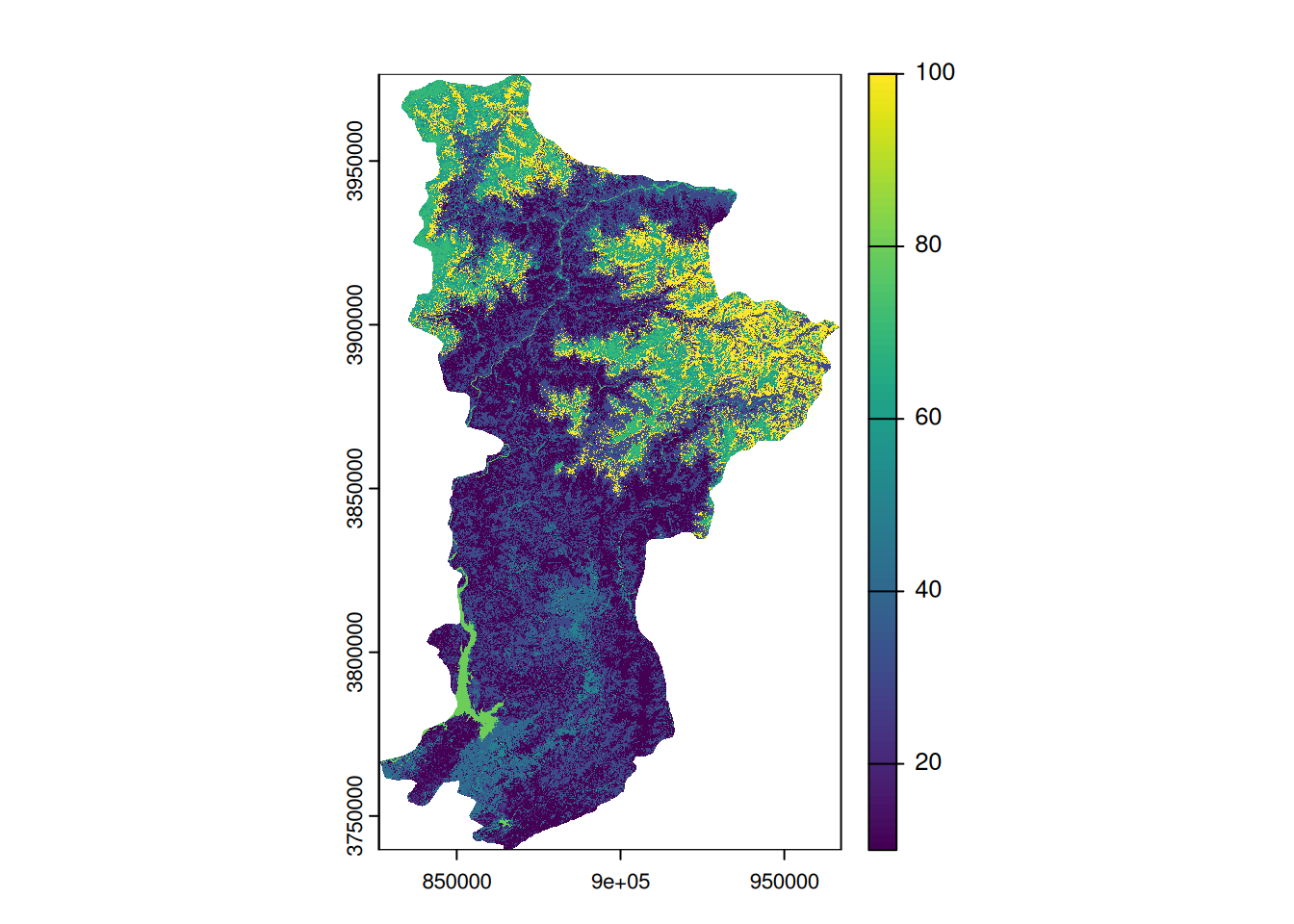

# we export this land cover raster
writeRaster(land_cover_hazara, './Data_processed/land_cover_hazara.tif', overwrite=TRUE)

In order to compare our land cover with the other layers, it is a good idea to vectorise this raster.

Vectorising a raster

In the world of GIS, we are used to working mainly with vector data. We will therefore vectorise our land cover raster. Each group of homogeneous pixels will be integrated into a polygon, one attribute of which will take the value of the pixels in the homogeneous group; in our case, this will be the class identifier.

# vectorisation of the land cover raster
land_cover_vect <- as.polygons(land_cover_hazara)
land_cover_vect

 class       : SpatVector 
 geometry    : polygons 
 dimensions  : 10, 1  (geometries, attributes)
 extent      : 826270.3, 967319.4, 3739588, 3976586  (xmin, xmax, ymin, ymax)
 coord. ref. : WGS 84 / UTM zone 42N (EPSG:32642) 
 names       : ESA_WorldCover
 type        :          <int>
 values      :             10
                           20
                           30

We can verify that our new layer contains an attribute in which we find the identifier for land cover classes. What is the name of this identifier? Using the first part of this documentation as a guide, rename this attribute with a relevant name (e.g. id_class).

Answer

To rename this attribute, we follow the following syntax.

names(land_cover_vect)[names(land_cover_vect) == 'ESA_WorldCover'] <- 'id_class'

Following the procedure described above, extract the forest polygons (class 10) and store them in a variable named forest_div. What syntax will you use? How many features are there in the resulting layer?

Answer

The extraction of forest polygons will be done according to an attribute selection on the id_class field.

forest_div <- land_cover_vect[land_cover_vect$id_class == 10, ]
forest_div

 class       : SpatVector 
 geometry    : polygons 
 dimensions  : 1, 1  (geometries, attributes)
 extent      : 826670.3, 963669.4, 3739588, 3966686  (xmin, xmax, ymin, ymax)
 coord. ref. : WGS 84 / UTM zone 42N (EPSG:32642) 
 names       : id_class
 type        :    <int>
 values      :       10

Although there are numerous forest patches, the layer contains only one entity. It is in fact a multi-part polygon.

What is the area of the vivision covered by forest? What percentage does this represent?

Answer

To answer this question, simply add an area attribute and convert it to square kilometres.

# we calculate the area of forest in km2
forest_div$area_km2 <- expanse(forest_div) / 1000000
# we grab this value into a variable
area_f <- forest_div$area_km2
# we calculate the percentage by comparing this value to the total area of the division
pc_f <- area_f / (expanse(hazara) / 1000000) * 100

In total, forests cover 5254.31 km² in our division, representing 30.81% of the division’s territory.

We now have a view of the forest at the division level via an automatic procedure. It is possible to repeat the process for another land cover type.

Your turn

What percentage of the Hazara division is covered by grassland?

Some geoprocessing techniques

One of the purposes of GIS is to combine different layers to create new data that answers a question. Geoprocessing allows different layers to be combined to create new data. Here, we will focus on the portions of division covered by forest cover in order to identify the most wooded tehsil in the divisions of Hazara, and we will also extract the portions of tehsils that are not covered by forest.

First we import the layer of tehsils of Hazara.

tehsil <- vect('./Data/hazara_tehsils.gpkg')

Which geoprocessing method will enable you to quantify the proportion of forest in each tehsil?

Answer

The geoprocessing operation used to extract the space occupied by two entities at once (in this case, the tehsils and the forest) is intersection.

Before performing the intersection itself, we will add an area attribute to the tehsils. This will enable us to calculate the proportion of forest per tehsil.

# if necessary we import the layer of tehsils
tehsil <- vect('./Data/hazara_tehsils.gpkg')
# we calculate the area of each tehsil in km2
tehsil$area_tehsil_km2 <- expanse(tehsil) / 1000000

# we intersect the tehsils and the forests
tehsil_forest <- intersect(tehsil, forest_div)

# we calculate the area of each patch of forest
tehsil_forest$area_km2 <- expanse(tehsil_forest) / 1000000

# we caclculate the percentage of forest in each tehsil
tehsil_forest$pc_forest <- (tehsil_forest$area_km2 / tehsil_forest$area_tehsil_km2) * 100
#tehsil_forest

This enables us to identify the most and least wooded tehsils (as a percentage).

# the tehsil with the max percentage of forest, its name and its percentage
tehsil_max <- tehsil_forest[tehsil_forest$pc_forest == max(tehsil_forest$pc_forest)]$`name:en`
pc_max <- tehsil_forest[tehsil_forest$pc_forest == max(tehsil_forest$pc_forest)]$pc_forest
# the tehsil with the min percentage of forest, its name and its percentage
tehsil_min <- tehsil_forest[tehsil_forest$pc_forest == min(tehsil_forest$pc_forest)]$`name:en`
pc_min <- tehsil_forest[tehsil_forest$pc_forest == min(tehsil_forest$pc_forest)]$pc_forest

The tehsil with the highest proportion of forest cover is Battera Kolai Tehsil with a forest cover percentage of 61.65, and the tehsil with the lowest proportion of forest cover is Murree Tehsil with a forest cover percentage of 0.27.

Your turn

Now do the reverse and extract the portions of tehsils that are not forested. You will need to use the difference geoprocessing tool.

Zonal statistics

The aim of the following manipulation is to calculate zonal altitude statistics by divisions. We will calculate the maximum altitude and average altitude per division. We begin by loading our division layer into our script.

library(terra)
# import of the division layer
pk_div <- vect('./Data/PK_admin_L2.gpkg')

:::

What is the CRS of this layer?

Answer

As seen in the first part, there is a terra function to obtain the CRS of a layer.

# CRS of the layer
crs(pk_div, describe=TRUE)

                   name authority  code
1 WGS 84 / UTM zone 42N      EPSG 32642
                                                                                                                                                                                         area
1 Between 66°E and 72°E, northern hemisphere between equator and 84°N, onshore and offshore. Afghanistan. India. Kazakhstan. Kyrgyzstan. Pakistan. Russian Federation. Tajikistan. Uzbekistan
         extent
1 66, 72, 0, 84

The layer is in WGS84/UTM Zone 42 North, which is relevant for our study. We can now load our DEM into R.

# import of the DEM
dem <- rast('./Data/GTopo_PK.tif')
# plotting
plot(dem)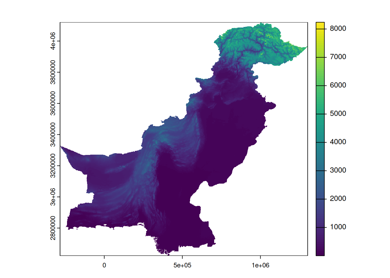

What is the CRS of this layer?

Answer

Similarly, it is easy to retrieve the CRS of a raster layer.

# CRS of the raster
crs(dem, describe=TRUE)

                   name authority  code
1 WGS 84 / UTM zone 42N      EPSG 32642
                                                                                                                                                                                         area
1 Between 66°E and 72°E, northern hemisphere between equator and 84°N, onshore and offshore. Afghanistan. India. Kazakhstan. Kyrgyzstan. Pakistan. Russian Federation. Tajikistan. Uzbekistan
         extent
1 66, 72, 0, 84

It may be interesting to look at the spatial resolution of our DEM.

# spatial resolution
res(dem)

[1] 852.4824 994.3244

The result contains two values, the size of a pixel in X and Y. Here, a pixel measures approximately 852.48 metres on each side.

We can now compare our DEM with the divisions. For example, we will calculate the average and maximum altitude per division. The terra function to use is extract. We add the option na.rm = TRUE so as not to take into account pixels without values in the raster.

# mean and max altitude
div_alti <- extract(dem, pk_div, fun=c('mean', 'max'), bind=TRUE, na.rm = TRUE)

What is the highest point in Pakistan according to our data? What can you tell us about it?

Answer

The highest point is the maximum value of the field containing the highest points by division.

# highest point
alti_max <- max(div_alti$max_GTopo_PK)

The highest point of our DEM rises to 8238, which does not correspond to the 8,611 m of Mont K2. This is normal, as we have pixels that average the altitude over the surface of each pixel, i.e. squares of 852.48 m by 994.32 m. So the peak of Mont K2 is averaged with the surrounding altitudes over approximately 50 hectares.

Is the division with the highest point in the territory the same as the division with the highest average elevation?

Answer

The division with the highest maximum point can be found by querying the max_GTopo_PK column.

# extraction of the division containing the highest point
div_highest <- div_alti[div_alti$max_GTopo_PK == max(div_alti$max_GTopo_PK)]
# we grab the name of this division
div_highest <- div_highest$NAME_2

The division containing the highest point is the division of Northern Areas. The division with the highest average is found in a similar manner.

# division with the highest average
div_mean_highest <- div_alti[div_alti$mean_GTopo_PK == max(div_alti$mean_GTopo_PK)]
div_mean_highest <- div_alti[div_alti$mean_GTopo_PK == max(div_alti$mean_GTopo_PK)]$NAME_2

This time, it is the division of Northern Areas.

Discretising a raster

We will now look at how to hide a raster according to a vector polygon. Let’s start by extracting a division of our choice.

# extraction of a division
div_xtr <- pk_div[pk_div$NAME_2 == 'Mardan']
plot(div_xtr)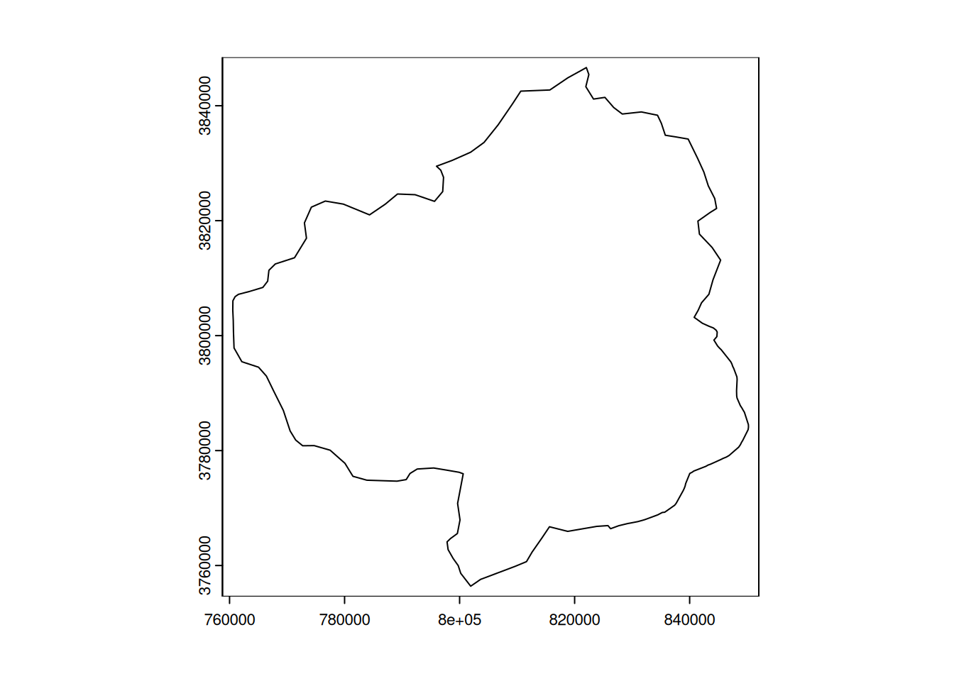

Next, two operations must be performed (in any order): cropping and masking. We can start by cropping our raster according to our division. This means that we remove all pixels from the raster that are not within the boundaries of our cropping polygon. This is equivalent to centring our raster. This is done using the crop function in terra.

# cropping of the raster
dem_xtr <- crop(dem, div_xtr)
plot(dem_xtr)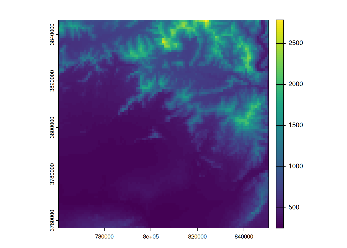

It is possible to export the result to your hard drive in .tif format.

# export of the raster
writeRaster(dem_xtr, './Data_processed/dem_xtr.tif', overwrite = TRUE)

Your turn

Practise extracting and exporting the DEM cropped and mask for a division of your choice.

Once the DEM has been extracted for a division, we can discretise our raster. For example, we can easily create a binary raster in which pixels above a certain altitude will be set to 1 and the others to 0. For this example, the threshold will be the average altitude of the division. Pixels above the average will be set to 1 and pixels below the average will be set to 0.

# we calculate the mean altitude of the raster
m <- global(dem_xtr, fun="mean", na.rm = TRUE) 
# we create a binary raster
dem_binary <- dem_xtr > m[[1]]
plot(dem_binary)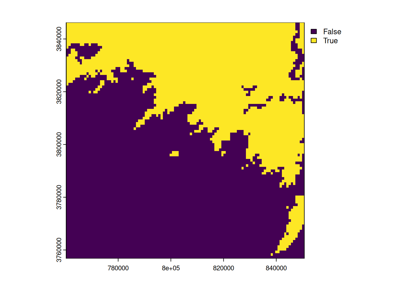

We obtain a binary raster with pixels set to True (1) and False (0) depending on whether they are above or below the threshold. We can count the number of pixels in each category and then multiply this number by the spatial resolution of a pixel. This gives us the area occupied by these two altitude categories. Here, we are doing what is called a zonal histogram.

# area of a pixel (m2)
area_pix <- res(dem_binary)[1] * res(dem_binary)[2]
# we calculate the frequencies of the pixels
f <- freq(dem_binary)
# we calculate the area of the altitude classes
area_alti_0 <- (f$count[f$value == 0] * area_pix) / 1000000
area_alti_1 <- (f$count[f$value == 1] * area_pix) / 1000000

The altitudes below the average in our division thus cover 4873.11 km² and those above 3213.42 km².

Raster to vector

In GIS, it is common to have to convert a raster file into a vector file in order to compare it with other layers. This conversion, also known as vectorisation, can be done using the as.polygons function in terra. Here, we will vectorise our binary raster in order to obtain a polygon corresponding to areas above the average altitude and a polygon for those below the average altitude.

# vectorisation of the binary raster
alti_vect <- as.polygons(dem_binary)
plot(alti_vect)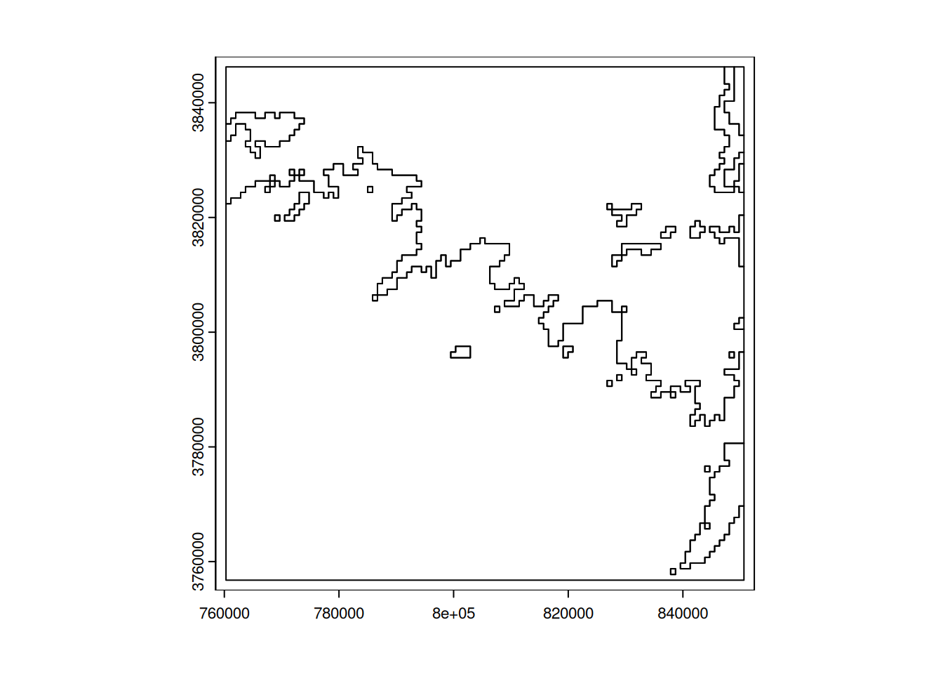

Add an attribute to this new layer in which you store the area in square kilometres for each zone. What do you notice in comparison with the areas calculated from the raster?

Answer

# we add a field with the area
alti_vect$area_km2 <- expanse(alti_vect) / 1000000
# we plot the attribute table
values(alti_vect)

  GTopo_PK area_km2
1        0 4866.085
2        1 3208.038

Ultimately, areas with above-average altitudes cover 3213.42 km² according to the raster layer and 3208.04 km² according to the vector layer. The two values are not identical because, by default, the expanse function for a vector layer calculates the area according to the ellipsoid, whereas the pixel resolution of the raster is given in the raster projection. The projection here is UTM Zone 42 North, a conformal projection that does not preserve areas.

Automation

The advantage of using a programming language is that it allows you to automate tasks. For example, what we did for one division can be run across all division in our division layer to produce a DEM raster for each division.

First, we can display all the division boundaries one by one. You can explore the boundaries by browsing the graphs in your RStudio Plots panel.

for(i in 1:length(pk_div)){
  plot(pk_div[i])
}

Now all we need to do is change the plot to what we want to do, for example, cut and mask the DEM for each division.

# cropping and masking of the DEM for each division
for(i in 1:length(pk_div)){
  dem_loop <- crop(dem, pk_div[i])
  dem_loop <- mask(dem_loop, pk_div[i])
  plot(dem_loop)
}

By changing the line plot(dem_loop), we could save the result of each division to the hard drive.