# basic GIS processings
# loading of the terra library
library(terra)Vector layer processing
Objectives of the first section
The aim of this section is to start manipulating vector data and performing basic but frequently used operations on it. We will be working on the divisions of Pakistan, focusing in particular on the populations of these divisions. By the end of this section, you will be able to perform the following operations in R:
- import a vector layer
- export a vector layer
- check the coordinate reference system (CRS) of a geographic layer
- perform an attribute join
- perform an attribute query on text or numbers
- group entities according to a common attribute
- perform a spatial query
- group entities according to a common field by calculating statistics
Data provided
For this exercise, we will use the following data:
- the layer of Pakistani Divisions in GeoPackage (PK_admin_L2.gpkg)
- the spreadsheet of census populations (PK_census.xlsx)
- the layer of the main waterways in Pakistan in GeoPackage (main_rivers_PK.gpkg)
Getting started
For processing spatial data, we will use the terra library. There are various libraries available for geomatics, but this one has the advantage of working with both types of objects (vector and raster). You can find the complete documentation online, but here we will only explore a few features. Install this library as explained in the introduction. Once terra is installed, simply call it by adding the following line at the top of your script.
We can now load our vector layer using the terra library. We load it into an object of type spatVector that we name pk_div. Note that the terra library supports many file formats. We could have provided it with a shapefile if our layer had been a .shp.
pk_div <- vect('./Data/PK_admin_L2.gpkg')
Formats
Pay attention to the path to your files. The path can be relative or absolute. Furthermore, in Windows, it is necessary to double the path separator like this // or reverse it **.
To verify the integrity of our layer, we can quickly trace it and display its properties and an extract from its attribute table.
plot(pk_div)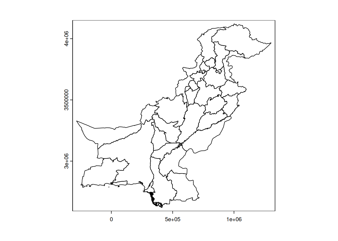
pk_div class : SpatVector
geometry : polygons
dimensions : 32, 4 (geometries, attributes)
extent : -283875.3, 1303036, 2621633, 4120742 (xmin, xmax, ymin, ymax)
source : PK_admin_L2.gpkg
coord. ref. : WGS 84 / UTM zone 42N (EPSG:32642)
names : COUNTRY NAME_1 NAME_2 TYPE_2
type : <chr> <chr> <chr> <chr>
values : Pakistan Azad Kashmir Azad Kashmir Division
Pakistan Balochistan Kalat Division
Pakistan Balochistan Makran DivisionWhat do the different properties mean?
Answer
The object is of class SpatVector, the stored geometries are polygons, and there are 32 of them with 4 attributes in the attribute table. The layer has a certain geographical extent in the WGS 84 / UTM zone 42N (EPSG:32642) coordinate system. Finally, we have the names of the different attributes as well as their types and an extract of the first 3 lines of the attribute table.
Attribute selections
Attribute tables are similar to dataframes, and the same type of operation can be performed on them. For example, it is possible to extract a division by name and isolate it in a new object.
# extraction of a division
my_div <- pk_div[pk_div$NAME_2 == 'Lahore', ]
my_div
class : SpatVector
geometry : polygons
dimensions : 1, 4 (geometries, attributes)
extent : 901711.9, 1043502, 3361318, 3558064 (xmin, xmax, ymin, ymax)
coord. ref. : WGS 84 / UTM zone 42N (EPSG:32642)
names : COUNTRY NAME_1 NAME_2 TYPE_2
type : <chr> <chr> <chr> <chr>
values : Pakistan Punjab Lahore Divisionplot(my_div)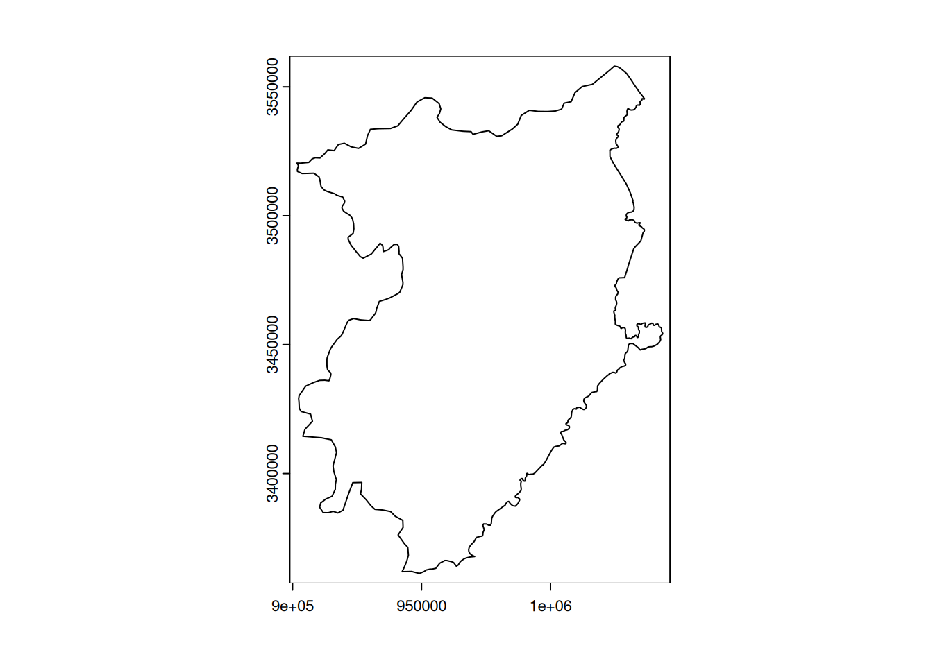
In the previous selection, we selected the division of Lahore and stored its polygon and associated attributes in a new variable named my_div.
Warning
By default, R is case-sensitive and sensitive to accents, so please be careful.
We can do the same to extract all the divisions in a given district For example, let’s extract the divisions in Punjab.
div_punj <- pk_div[pk_div$NAME_1 == 'Punjab', ]
div_punj
class : SpatVector
geometry : polygons
dimensions : 8, 4 (geometries, attributes)
extent : 525600, 1100170, 3065214, 3774012 (xmin, xmax, ymin, ymax)
coord. ref. : WGS 84 / UTM zone 42N (EPSG:32642)
names : COUNTRY NAME_1 NAME_2 TYPE_2
type : <chr> <chr> <chr> <chr>
values : Pakistan Punjab Bahawalpur Division
Pakistan Punjab Dera Ghazi Khan Division
Pakistan Punjab Faisalabad Divisionplot(div_punj)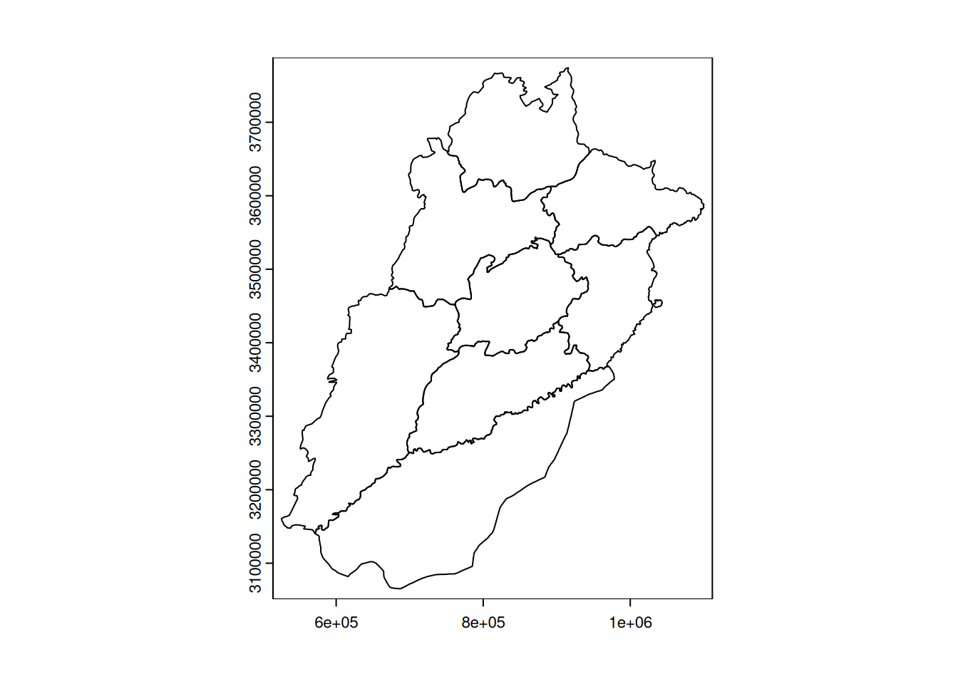
Your turn
Extract a division of your choice, then all divisions in a district.
As we can see, our layer of divisions does not contain any information about population. However, we do have this information in the spreadsheet provided, PK_census.xlsx. We will therefore be able to perform an attribute join. We will begin by loading the spreadsheet.
library(readxl)
tab_div <- read_excel('./Data/PK_census.xlsx')
We create a new variable, of type dataframe, containing the division populations.
Attribute joins
To perform an attribute join, both tables must have a common field of the same type. What is the field common to both tables?
Answer
The common field is the division field of the spreadsheet file and NAME_2 from the vector file, which are text fields.
Before performing the join, we will create an intermediate dataframe that will only contain the attributes relevant to the join. This will prevent us from having duplicate fields in the join result. From the tab_div dataframe, we will only keep the Division and Census_2017 fields.
tab_div_xtr <- tab_div[c('Division', 'Census_2017')]We then join our pk_div vector with this dataframe, filtered according to the common field. The terra function to use is merge.
pk_div_pop <- terra::merge(pk_div, tab_div_xtr, by.x='NAME_2', by.y='Division')We now have a vector layer of divisions with population information. This allows us to query divisions according to their population.
# divisions with less than 1 000 000 inh.
pk_div_small_pop <- pk_div_pop[pk_div_pop$Census_2017 < 1000000, ]
The same applies to divisions with more than 2 000 000 inhabitants.
# divisions with more than 2 000 000 inh.
pk_div_large_pop <- pk_div_pop[pk_div_pop$Census_2017 > 2000000, ]
Your turn
Select divisions with a population between 1,000,000 and 2,000,000 inhabitants. Then select divisions with more than 2,000,000 inhabitants in the Balochistan district.
Answer
The following two lines answer the two questions respectively.
pk_div_xtr <- pk_div_pop[pk_div_pop$Census_2017 > 1000000 & pk_div_pop$Census_2017 < 2000000, ]
pk_div_xtr2 <- pk_div_pop[pk_div_pop$NAME_1 == 'Balochistan' & pk_div_pop$Census_2017 > 2000000, ]
Attribute field calculations
It is very common to have to add new fields to an attribute table. When working with administrative entities, or polygons in general, calculating the area of each entity is a very common operation. We will add an attribute called area_km2 in which we will store the area in square kilometres of each division. The function to use in the terra library is called expanse. This function has the particularity of calculating the area of each entity directly on the ellipsoid used in the reference coordinate system. By default, this function does not take into account the map projection. It is therefore not necessary to consider the nature of the projection (conformal or equivalent). However, the base unit is square metres, so the area must be converted into square kilometres.
# add a field to store the area
pk_div_pop$area_km2 <- expanse(pk_div_pop) / 1000000
Your turn
What is the name of the largest division?
Answer
With the first line, we select the attributes of the largest division With the second line, we select only its name.
pk_div_pop[pk_div_pop$area_km2 == max(pk_div_pop$area_km2)] class : SpatVector
geometry : polygons
dimensions : 1, 6 (geometries, attributes)
extent : -116300.6, 357234.4, 2754998, 3346311 (xmin, xmax, ymin, ymax)
coord. ref. : WGS 84 / UTM zone 42N (EPSG:32642)
names : NAME_2 COUNTRY NAME_1 TYPE_2 Census_2017 area_km2
type : <chr> <chr> <chr> <chr> <num> <num>
values : Kalat Pakistan Balochistan Division 2.175e+06 1.379e+05pk_div_pop[pk_div_pop$area_km2 == max(pk_div_pop$area_km2)]$NAME_2[1] "Kalat"Now that we have the area of each division and the population of each division, we are eager to calculate the population density for each division. Calculate these densities in a field named density_inh. What is the average density of the Pakistani divisions?
Answer
Density is simply the ratio between the number of inhabitants and the surface area in square kilometres of each division.
pk_div_pop$density_inh <- pk_div_pop$Census_2017 / pk_div_pop$area_km2
# densité moyenne
mean(pk_div_pop$density_inh)
[1] 672.7393We can export the final layer of divisions attached to populations.
# export of the layer of divisions with census
writeVector(pk_div_pop, './Data_processed/divisions_PK_pop.gpkg', overwrite=TRUE)
Grouping entities by field
Grouping entities by common values in a field in the attribute table is a common operation in GIS. Here, for example, we have a layer of polygons representing the divisions of Pakistan, for which we know the district to which they belong based on the NAME_1 field. We are going to create a new SpatVector object, named district, which will contain the polygons of the districts of Pakistan. We will thus group the polygons of the divisions according to the NAME_1 field. We just need to pay attention to the attribute fields that we want to keep. All text fields related to divisions will no longer be relevant at the districts level, so we can remove them. However, we can group quantitative fields, such as population, area and density, according to a relevant grouping statistic. In your opinion, which statistics should we use for these three fields?
Answer
It is important to note that some quantities can be averaged and others summed. For example, the population can be summed to obtain the total population of each district. The same applies to surface area. It would not be wrong to calculate the averages of these two fields, but we would obtain the average division population of the district and the average division area of the district, which is not necessarily interesting. The field containing the densities, on the other hand, cannot be summed. A sum of density has no mathematical meaning. We could average it to obtain the average division density for the district, but this is not very interesting. Therefore, we will recalculate the district density retrospectively.
Aggregation can be performed using the aggregate function in terra.
district <- aggregate(pk_div_pop, by='NAME_1', dissolve=TRUE, fun="sum")
district
class : SpatVector
geometry : polygons
dimensions : 8, 8 (geometries, attributes)
extent : -283875.3, 1303036, 2621633, 4120742 (xmin, xmax, ymin, ymax)
coord. ref. : WGS 84 / UTM zone 42N (EPSG:32642)
names : NAME_1 sum_Census_2017 sum_area_km2 sum_density_inh
type : <chr> <num> <num> <num>
values : Azad Kashmir 4.032e+06 1.39e+04 290.1
Balochistan 1.086e+07 3.445e+05 255.4
Federally Admi~ 5.002e+06 2.504e+04 199.8
NAME_2 COUNTRY TYPE_2 agg_n
<chr> <chr> <chr> <int>
Azad Kashmir Pakistan Division 1
NA Pakistan Division 6
F.A.T.A. Pakistan Division 1The fields relating to divisions sum_density_inh, NAME_2 and TYPE_2 are no longer useful, so we can delete them. We can also rename certain fields with more explicit names. We will take this opportunity to recalculate the population density at the division level.
# we remove useless fields by their names
district$sum_density_inh <- NULL
district$NAME_2 <- NULL
district$TYPE_2 <- NULL
# we rename some fields
names(district)[names(district) == 'sum_Census_2017'] <- 'Population_district'
names(district)[names(district) == 'sum_area_km2'] <- 'area_district_km2'
names(district)[names(district) == 'agg_n'] <- 'nb_div_district'
# we calculate the population density for each district
district$density_inh <- district$Population_district / district$area_district_km2
We now have a layer of districts with a relevant attribute table. Once we have this layer, we can export it as a GeoPackage so that we can open it in GIS software or another tool.
writeVector(district, './Data_processed/district_PK.gpkg', overwrite=TRUE)Spatial selections
We will now select divisions according to a spatial criterion for a given division. For example, we will extract the Dera Ismail Khan division from our pk_div_pop variable containing all divisions, then we will select all divisions in neighbouring divisions that touch the Dera Ismail Khan division.
# extraction of the Dera Ismail Khan division
div_DIKhan <- pk_div_pop[pk_div_pop$NAME_2 == 'Dera Ismail Khan', ]
# if we want to export the polygon of this vivision, uncomment the next line
#writeVector(div_DIKhan, './Data_processed/div_DIKhan.gpkg', overwrite=TRUE)
The spatial selection is then carried out in two stages. First, for each division, we check whether or not (True or False) it borders our division Then, from among all the divisions, we select those that are True.
# touching or not
relation_touche <- relate(pk_div_pop, div_DIKhan, relation="touches")
# selection of divisions that respond True to the fact of touching
div_border <- pk_div_pop[relation_touche[,1], ]
Your turn
How many divisions are bordering the Punjab district?
Answer
As before, this selection is done in three steps: creation of a SpatVector variable for the Punjab district, then assignment of True or False depending on whether or not a division touches this polygon, and finally extraction of the polygons with True.
# the Punjab polygon
punjab <- district[district$NAME_1 == 'Punjab', ]
# the divisions bordering or not the Punjab
relation_touche <- relate(pk_div_pop, punjab, relation="touches")
# selection of divisions that respond True to the fact of touching Punjab
div_border_punjab <- pk_div_pop[relation_touche[,1], ]
Divisions and hydrography
We will now link the divisions with the main waterways. First, let’s load the hydrographic network provided in the main_rivers_PK.gpkg file. This layer lists the main waterways of Pakistan.
hydro <- vect('./Data/main_rivers_PK.gpkg')What is the type of geometry of this layer?
Answer
To find out, simply enter the name of the variable in the console and the basic information will be displayed.
hydro class : SpatVector
geometry : lines
dimensions : 12, 2 (geometries, attributes)
extent : 67.53232, 81.63975, 23.90949, 35.84284 (xmin, xmax, ymin, ymax)
source : main_rivers_PK.gpkg (ne_10m_rivers_lake_centerlines)
coord. ref. : lon/lat WGS 84 (EPSG:4326)
names : name name_ur
type : <chr> <chr>
values : Ravi دریائے راوی
Beas دریائے بیاس
Beas دریائے بیاسThe layer contains lines (geometry : lines).
What is the name of the field containing the name of the rivers?
Answer
To display the names of all attributes in the layer, we use the names function.
names(hydro)[1] "name" "name_ur"The field containing the name of the rivers of each watercourse is named name.
What is the reference coordinate system for this hydrography layer? What do you recommend?
Answer
We can display the SCR of a layer using the crs function in terra and the describe=TRUE option.
crs(hydro, describe=TRUE) name authority code area extent
1 WGS 84 EPSG 4326 World -180, 180, -90, 90Our layer is unprojected and uses the WGS84 global system. It is therefore necessary to reproject it into the UTM zone of Pakistan WGS84/UTM Zone 42 North system (ESPG:32642) before crossing it with our other layers. This is easily done using the project function in terra.
# we create a new layer in the UTM Zone 42 North system
hydro_utm42 <- project(hydro, 'EPSG:32642')
We now have the layer of the main Pakistani waterways in the correct SCR. We can therefore compare it with our other layers of divisions or districts. It may be interesting to know the total population of the divisions crossed by a major waterway. To extract the divisions crossed by a major waterway, which GIS function will you use?
Answer
This type of processing involves spatial selection. We will link the layer of divisions and the layer of watercourses using the same principle as before, but with the correct geometric predicate.
# identification of the divisions crossed by a waterway
relation_hydro <- relate(pk_div_pop, hydro_utm42, relation="intersects")
# selection of divisions that respond True to the fact of being crossed by a waterway
relation_hydro <- cbind(relation_hydro, apply(relation_hydro, 1, any))
div_hydro <- pk_div_pop[relation_hydro[,ncol(relation_hydro)]]
You will notice that there is an extra line compared to before. This is necessary, otherwise only the first division crossed by a watercourse will be selected. Accept the syntax as it is.
We can verify the result by viewing it and exporting the layer created.
plot(div_hydro)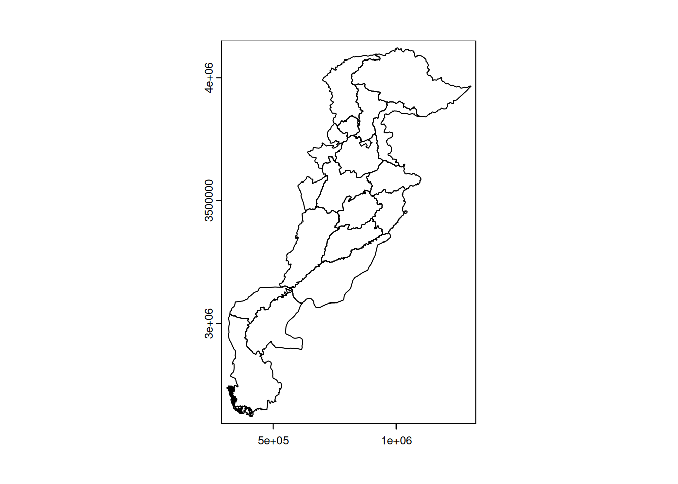
writeVector(div_hydro, './Data_processed/divisions_hydro.gpkg', overwrite = TRUE)The total population of divisions crossed by watercourses can be calculated from this layer.
div_hydro <- sum(div_hydro$Census_2017)
div_hydro
[1] 163315219In total, 1.6331522^{8} inhabitants live in a division crossed by a main watercourse.
After these few basic manipulations on vector layers, we will see in the second part how to perform new geoprocessing operations and interact with raster data.